- CFA Exams
- 2026 Level II
- Topic 1. Quantitative Methods
- Learning Module 5. Time-Series Analysis
- Subject 2. Autoregressive (AR) Time-Series Models
Why should I choose AnalystNotes?
Simply put: AnalystNotes offers the best value and the best product available to help you pass your exams.
Subject 2. Autoregressive (AR) Time-Series Models PDF Download
When the dependent variable is regressed against one or more lagged values of itself, the resultant model is called as an Autoregressive Model (AR). Autoregressive models are abbreviated AR(p) models, where p is known as the order of the model.
In the AR model, we abandon the dependent (y) and independent (x) notion and use xt since there is no longer a difference.
Chain Rule of Forecasting
The chain rule of forecasting can be used to derive multi-period forecasts using an AR(p) model. It involves calculating a one-step-ahead forecast before a two-step ahead forecast as the independent variable is a lagged value of the dependent variable.
The one-period-ahead forecast of a variable xt from an AR(1) model made in period t for period t + 1 is x̂t+1 = b̂0 + b̂1 xt.
This forecast can be used to create the two-period-ahead forecast from the model made in period t, x̂t+2 = b̂0 + b̂1 xt+1.
Similar results hold for AR(p) models.
Example
Given an AR model where b̂0 = 4 and b̂1 = 3, if x0 = 2, the one-step-ahead forecast of x̂ 1 is closest to x̂ 1 = 4 + 3 x 2 = 10, and the two-step ahead forecast of x̂2 is closest = 4 + 3 x 10 = 34.
Residual Autocorrelation
If the residuals have significant autocorrelation, the AR model that produced the residuals is not the best model for the time series being analyzed. We can estimate an AR model using ordinary least squares (OLS) if the time series is covariance stationary and the errors are uncorrelated. Unfortunately, our previous DW test statistic is invalid when the independent variables include past values of the dependent variable. Residual autocorrelations drag to '0' as the no. of lags increases.
To test whether an AR model is correctly specified, the following steps are followed:
- Estimate the autoregressive model and calculate the residuals.
Calculate the autocorrelations of the residuals; i.e. the level of correlation between the forecast errors from one period to the next.- Perform a t-test to check if the autocorrelations are statistically different from 0.
The Mean Reversion
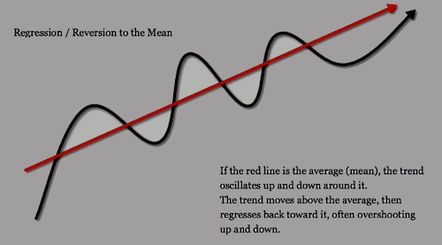
Mean reversion is a property of a time series where the values tend to move back towards a long-term average or mean over time. In autoregressive models, mean reversion is the assumption that the current value of a time series is a linear function of its past values and a white noise term, and that the past values of the time series are correlated to the current value.

In other words, if the current value of the time series is above or below the long-term average, it will tend to move back towards the average over time.
To calculate the mean reverting level: xt = b0/(1 - b1)
The value of an AR(1) model will tend to:
- remain the same if xt = b0/(1 - b1)
- increase if xt < b0/(1 - b1)
- decrease if xt > b0/(1 - b1)
Mean reversion is often used in finance to model the behavior of financial instruments such as stocks or currencies.
Multiperiod Forecasts
In-sample forecasts are the in-sample predicted values from the estimated time-series model. Errors: yt - ŷt, where t is an observation within the sample period.
Out-of-sample forecasts are the forecasts made outside of the sample period. Out-of-sample forecast accuracy is important because the future is always out-of-sample.
A model's accuracy in forecasting out-of-sample values is assessed using the root mean squared error (RMSE), which is the square root of the mean squared error. A smaller RMSE implies greater forecast accuracy and better predictive power.
Example
Table below gives the actual change in the Log of Sales of Cisco Systems from 1Q: 2001 to 4Q: 2001, along with the forecasts from the regression model Δln (Salest) = 0.0661 + 0.4698 x Δln (Salest-1) estimated using data from 3Q: 1991 to 4Q: 2000. Note the observations after the fourth quarter of 2000 are out-of-sample.

Calculate the RMSE for the out-of-sample forecast errors.

User Contributed Comments 1
| User | Comment |
|---|---|
| alai2008 | The point is that we estimate models that use as independent variable a previous value of the dependent variable. I.e. X = 7 +2 x Xt-1 |

I used your notes and passed ... highly recommended!

Lauren
My Own Flashcard
No flashcard found. Add a private flashcard for the subject.
Add