- CFA Exams
- 2026 Level II
- Topic 1. Quantitative Methods
- Learning Module 5. Time-Series Analysis
- Subject 1. Trend Models
Seeing is believing!
Before you order, simply sign up for a free user account and in seconds you'll be experiencing the best in CFA exam preparation.
Subject 1. Trend Models PDF Download
Time Series is a set of observations on a variable's outcomes in different time periods e.g. quarterly sales for a particular company during the past 5 years.
Time series models explain the past and predict the future of a time series using a trend, which is a long-term pattern in a specific direction.
Linear Trend Model
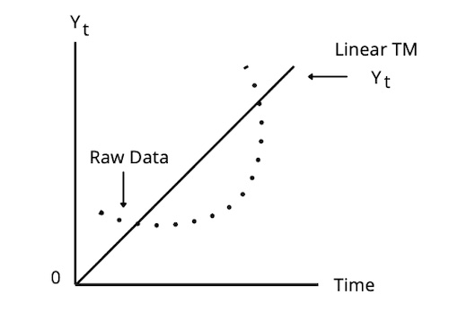
In a linear trend, the dependent variable changes at a constant amount with time. Consider a time series with a linear trend. The value of the time series at time t can be expressed as: yt = b0 + b1 (t) + εt, where t = 1,2,3,...T
A Linear Trend is a time series pattern that can be graphed using a straight line.

Time series that tend to grow by a constant amount from period to period should be modeled by linear trend models.
The predicted trend value of a time series in period t is b̂0 + b̂1 t in a linear trend model.
Log-Linear Trend Model
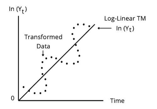
Time series that tend to grow at a constant rate (exponential growth) should be modeled by log-linear trend models: yt = eb0 + b1 (t) + εt, where t = 1,2,3,...T

Limitations of Trend Models
Trend models often do not completely capture the behavior of a time series, as he error terms may be correlated. This violates the linear regression assumption that residuals are uncorrelated with each other (serial correlation).
Serial correlation makes the linear regression estimates inconsistent and invalid. Serial correlation can be detected by performing a Durbin-Watson test. If the Durbin-Watson statistic from a trend model differs significantly from 2, indicating serial correlation, we need to build a different kind of model.
We can correct serial correlation by transforming the data or using other regression models such as an autoregressive model.
Covariance Stationary Property
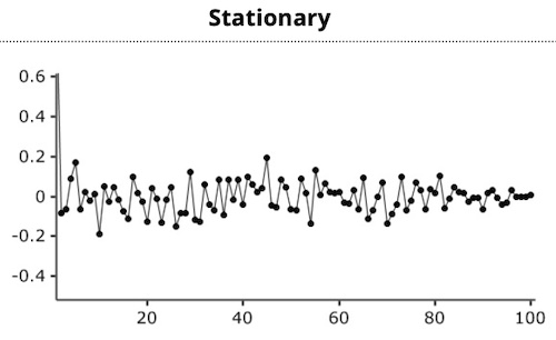
A time series is covariance stationary if its mean, variances and covariances with lagged and leading values don't change over time.

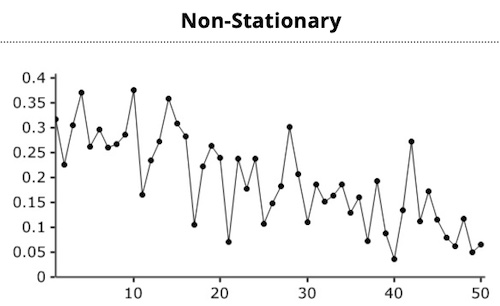
Data points are often non-stationary or have means, variances and covariances that change over time. e.g. trends, cycles, random walks or combinations of three.

Time series is covariance stationary if it satisfies the following three conditions:
- Constant and finite expected value.
- Constant and finite variance. The time series' volatility around its mean doesn't change over time.
- Constant and finite covariance between values at any given lag.
Note both 2 and 3 indicates the covariance of a random variable with itself is its variance: Covariance(yt, yt) = Var(yt)
Inspection of a nonstationary time-series plot may reveal an upward or downward trend (nonconstant mean) and/or nonconstant variance. In order to receive consistent-reliable results the non-stationary data needs to be transformed into stationary data. The use of linear regression to estimate an autoregressive time-series model is not valid unless the time series is covariance stationary.
User Contributed Comments 0
You need to log in first to add your comment.

I am happy to say that I passed! Your study notes certainly helped prepare me for what was the most difficult exam I had ever taken.

Andrea Schildbach
My Own Flashcard
No flashcard found. Add a private flashcard for the subject.
Add